


About PastML
PastML infers ancestral characters on a rooted phylogenetic tree with annotated tips, using maximum likelihood or parsimony. The result is then visualised as a zoomable html map.
Input data
Once you decide to run a PastML analysis, you will be asked for two files:
- a rooted tree;
- an annotation table specifying tip states.
Tree
The input tree should be in Newick format. It can be inferred with your favourite tool, e.g. PhyML, RAxML, FastTree, IQTree, or Beast2. Once inferred the tree must be rooted (with an outgroup or with dates, e.g. using gotree or LSD, etc.). The tree can (but does not have to) be dated.
Annotation table
The annotation table should be in CSV format (with your favourite separator character). Its first line must contain a header, specifying column names. One of the columns must contain the tip ids (in exactly the same format as used in the tree), and there must be at least one (or more) column(s) containing tip states for character(s) whose ancestral states are to be reconstructed with PastML. The characters to be analysed with PastML should be discrete, e.g. countries, presence/absence of a mutation, nucleotide value at a certain position, etc. The table may contain other columns that will not be used in PastML analysis. You will be asked to specify which of your table columns contains what, once you've uploaded the tree and the table.
If a state of a certain tip is unknown, it can be either omitted from the table or left blank. It will be estimated during PastML analysis. To restrict a tip state to several possibilities (e.g. UK or France) add multiple columns with this tip id in the annotation file, each containing a possible state (e.g. one columns for UK, and one for France). If states of some of the internal nodes are known, they can be specified in the same manner as tip states, but note that the input tree in that case should contain internal node names.
Example
Let's look at a toy data set with a four-tip tree ((t1:0.2,t2:0.4)n1:0.9,(t3:0.2,t4:0.6)n2:0.3)root; (in newick format, with internal nodes named), and the following annotation table:
| ID | Country | Continent | Other data |
|---|---|---|---|
| t1 | China | Asia | 4.37 |
| t2 | UK | Europe | 1.23 |
| t2 | France | Europe | 1.23 |
| t3 | Asia | 3.25 | |
| n1 | UK |
Column ID contains tree node ids, columns Country and Continent can be used for ancestral character reconstruction by PastML, and column Other data seems to contain continuous data that cannot be analysed with PastML. Tip t1 is annotated with Country:China and Continent:Asia, tip t2 with Country:UK or France and Continent:Europe, for tip t3 Country is unknown (and will be inferred by PastML), but it is annotated with Continent:Asia, finally for the internal node n1 Continent is unknown, but Country is fixed to UK. For the other nodes (tip t4, internal node n2, and root) their locations are unknown and can be inferred by PastML.
Ancestral character reconstruction (ACR)
PastML can reconstruct ancestral states using two types of methods: maximum likelihood or maximum parsimony.
Maximum Parsimony (MP) methods
MP methods aim to minimize the number of state changes in the tree. They are very quick but not very accurate, e.g. they do not take into account branch lengths. We provide three MP methods: DOWNPASS, ACCTRAN, and DELTRAN.
DOWNPASS
DOWNPASS [Maddison and Maddison, 2003] performs two tree traversals: bottom-up and top-down, at the end of which it calculates the most parsimonious states of ancestral nodes based on the information from the whole tree. However some of the nodes might be not completely resolved due to multiple parsimonious solutions.
ACCTRAN
ACCTRAN (accelerated transformation) [Farris, 1970] reduces the number of node state ambiguities by forcing the state changes to be performed as close to the root as possible, and therefore prioritises the reverse mutations.
DELTRAN
DELTRAN (delayed transformation) [Swofford and Maddison, 1987] reduces the number of node state ambiguities by making the changes as close to the tips as possible, hence prioritizing parallel mutations.
Maximum Likelihood (ML) methods
ML approaches are based on probabilistic models of character evolution along tree branches. From a theoretical standpoint, ML methods have some optimality guaranty [Zhang and Nei, 1997, Gascuel and Steel, 2014], at least in the absence of model violation. We provide three ML methods: maximum a posteriori (MAP), Joint, and marginal posterior probabilities approximation (MPPA, recommended).
MAP
MAP (maximum a posteriori) computes the marginal posterior probabilities of every state for each of the tree nodes, based on the information from the whole tree, i.e. tip states and branch lengths (obtained via two tree traversals: bottom-up, and then top-down). MAP then chooses a state with the highest posterior probability for each node, independently from one node to another. This could induce globally inconsistent scenarios (typically: two very close nodes with incompatible predictions).
JOINT
While MAP chooses predicted states based on all possible scenarios, Joint method [Pupko et al., 2000] reconstructs the states of the scenario with the highest likelihood.
MPPA (recommended)
MAP and Joint methods choose one state per node and do not reflect the fact that with real data and large trees, billions of scenarios may have similar posterior probabilities. Based on the marginal posterior probabilities, MPPA (marginal posterior probabilities approximation) chooses for every node a subset of likely states that minimizes the prediction error measured by the Brier score. It therefore sometimes keeps multiple state predictions per node but only when they have similar and high probabilities. Note however that the states not kept by MPPA might still be significant despite being less probable -- to check marginal probabilities of each state on a node consult the output marginal probabilities file (can be downloaded via the button below each compressed visualisation).
Character evolution models
We provide three models of character evolution that differ in the way the equilibrium frequencies of states are calculated: JC, F81 (recommended), and EFT (estimate-from-tips, not recommended).
JC
With JC model [Jukes and Cantor, 1969] all frequencies, and therefore rates of changes from state i to state j (i ≠ j) are equal.
F81 (recommended)
With F81 model [Felsenstein, 1981], the rate of changes from i to j (i ≠ j) is proportional to the equilibrium frequency of j. The equilibrium frequencies are optimised.
EFT
With EFT (estimate-from-tips) model, the equilibrium frequencies are calculated based on the tip state proportions, the rate of changes from i to j (i ≠ j) is proportional to the equilibrium frequency of j.
Visualisation
Once the ACR is performed, we visualise a compressed representation of the ancestral scenarios, which highlights the main facts and hides minor details. This representation is calculated in two steps: (i) vertical merge that clusters together the parts of the tree where no state change happens, and (ii) horizontal merge that clusters independent events of the same kind. For large trees two additional steps might be applied: relaxed merge and trimming.
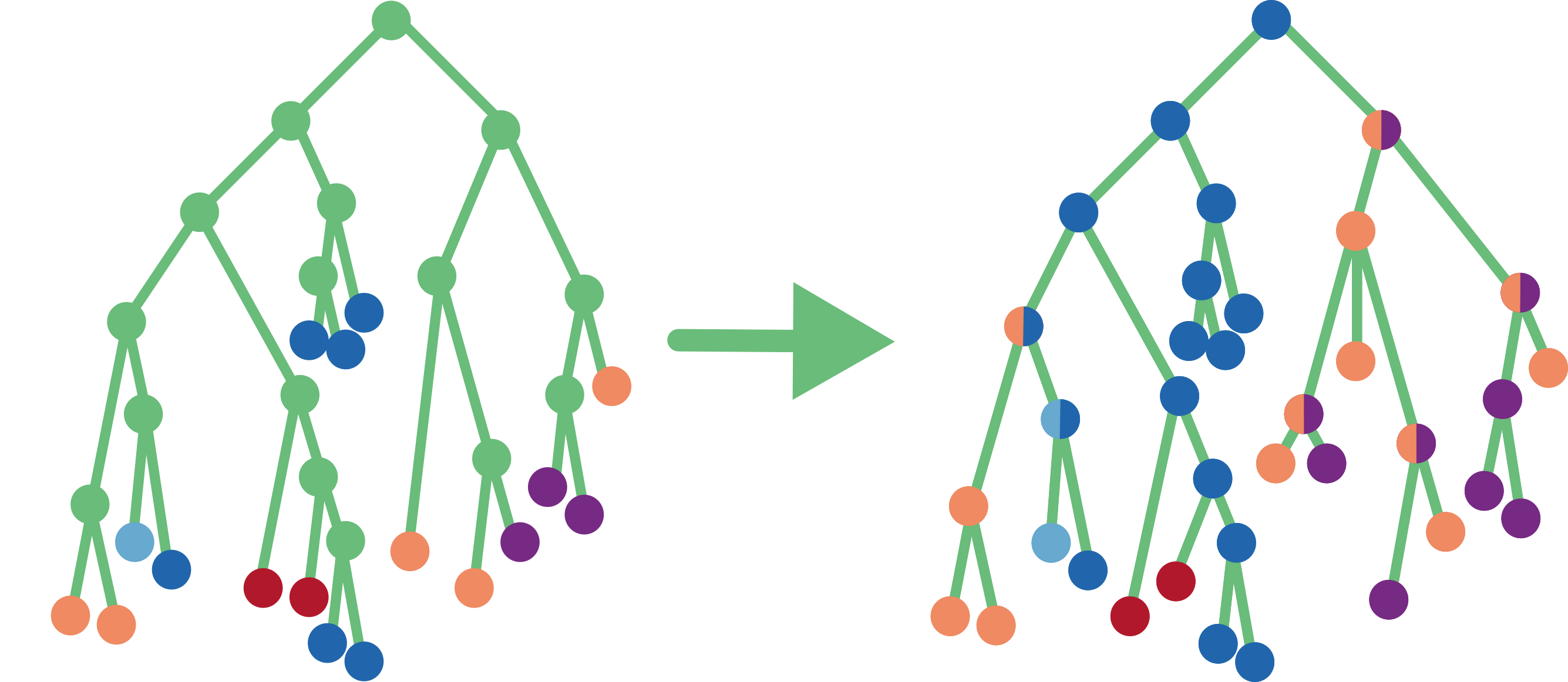
Vertical merge
While there exists a parent-child couple such that the parent’s set of predicted states is the same as the child’s one, we merge them. Once done, we compute the size of so-obtained clusters as the number of tips of the initial tree contained in them. Accordingly, in the initial tree each tip has a size of 1, each internal node has a size of 0, and when merging two nodes we sum their sizes.
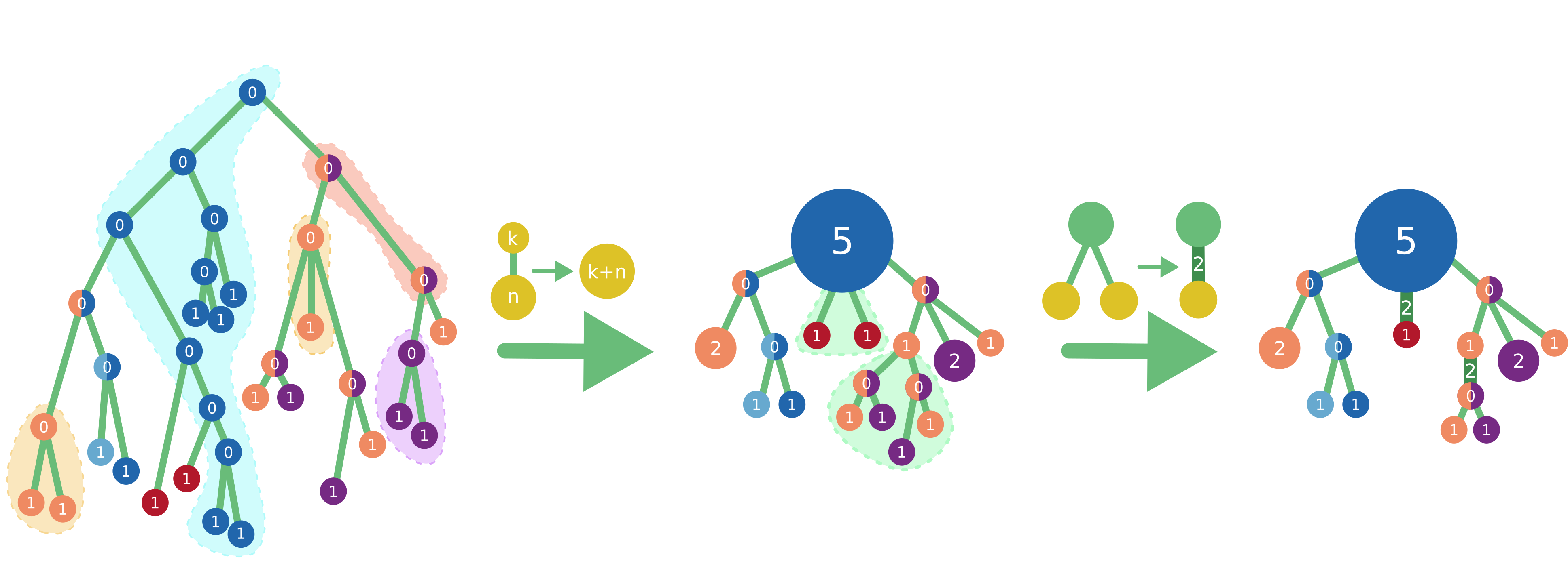
Horizontal merge
Starting at the root and going top-down towards the tips, at each node we compare its child subtrees. If two or more identical subtrees are found, we keep just one representative and assign their number to the size of the branch that connects the kept subtree to the current node. Hence a branch size corresponds to the number of times its subtree is found in the initial tree. Before the horizontal merge all branches have size 1.
Two trees are considered identical if they have the same topology and their corresponding nodes have the same state(s) and sizes. For example, two trees are identical if they are both cherries (a parent node with two tip children) with a parent in state A of size 3, a child in state B of size 2, and the other child in state C of size 1. However, those trees will not be identical to any non-cherry tree, or to a cherry with a parent not in state A, or to a cherry with the B-child of size 6, etc.
Relaxed merge and trimming
For large trees with many state changes even after the compression the visualization might contain too many details. To address this issue, we limit the number of tips shown in the compressed tree to about 15, which is achieved by performing a relaxed horizontal merge and hiding less important nodes.
In a relaxed horizontal merge, the definition of identical trees for the horizontal merge is updated: instead of requiring identical sizes of the corresponding nodes, we allow for nodes of sizes of the same order (log10); for instance, now a node in state A of size 3 can correspond to a node in state A of any size between 1 and 9, and a node in state B of size 25 can correspond to a node in state B of any size between 10 and 99.
If even after a relaxed horizontal merge the compressed representation contains too many details, we trim less important tips as follows. For each node we calculate its importance by multiplying its size by the sizes of all the branches on the path to the root of its branch, therefore obtaining the number of tips of the original tree that are represented by this node; for instance, a node leaf of size 2 connected to the root via branches of sizes 1, 3, and 5 gets an importance of 30. We call a node blocked by its descendant if its importance is smaller than the descendant’s one. The intuition behind is that this node cannot be removed from the tree unless the importance threshold allows to remove its descendant first. We then set the cut-off threshold to the 15-th largest non-blocked node’s importance, and iteratively trim all tips with smaller importance (once a tip is removed its parent becomes an unblocked tip itself and is also considered for trimming). Finally, we rerun relaxed horizontal merge as some of the previously different topologies might have become identical after trimming.
Multiple column analysis
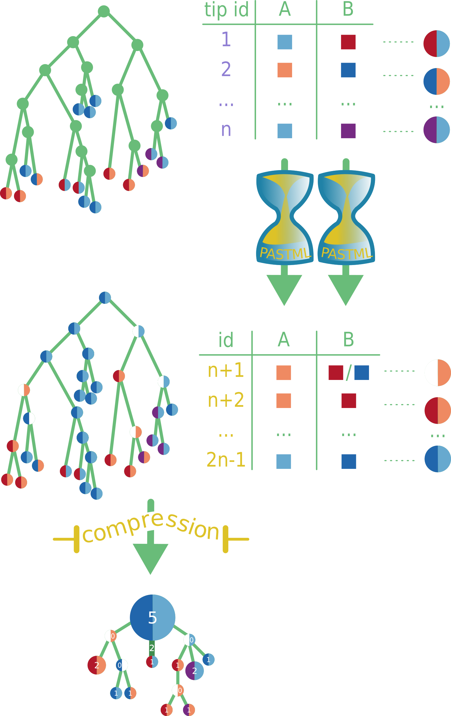
When multiple columns are selected for ACR analysis, we apply ACR independently to each character to obtain its ancestral states, and visualize each character on the tree nodes as sectors. If we could not choose a unique state for a character, we keep the corresponding sector uncolored (i.e. white). Once the tree is colored and each node is assigned its combined states (pie of colors), we compress the tree as described in the previous section.
Timeline
A slider is added to the right of the visualisation that allows to navigate in time. By default the time is measured in distance to the root, however if the input tree is dated (i.e. its branch lengths are specified in time units), and the root date has been specified by the user, the time is shown as dates. Three types of timeline can be chosen: sampled, nodes, and LTT. They differ in the elements of the tree that get hidden as the slider position is changed.
sampled
All the lineages sampled after the timepoint selected on the slider are hidden.
nodes
All the nodes with a more recent date/larger distance to root than the one selected on the slider are hidden.
LTT
All the nodes whose branch started after the timepoint selected on the slider are hidden, and the external branches are cut to the specified date/distance to root if needed.